Using machine learning and computer vision to automate the diagnosis of diabetic retinopathy from clinical eye images.
Published
August 1, 2019
1 Diabetic Retinopathy - Detecting Blindness
1.0.1 APTOS 2019 Blindness
Diabetic Retinopathy is a disease that affects the retina of the eye. Millions around the world suffer from this disease.
Currently, diagnosis happens through the use of a technique called fundus photography, which involves photographing the rear of the eye.
Medical screening for diabetic retinopathy occurs around the world, but is more difficult for people living in rural areas.
Using machine learning and computer vision, we attempt to automate the process of diagnosis, which currently is manually being performed doctors.
On Kaggle (https://www.kaggle.com/c/aptos2019-blindness-detection/data and https://www.kaggle.com/c/diabetic-retinopathy-detection) we will have access to a dataset of tens of thousands of real-world clinical images of both healthy patients and pateints with the disease, and labelled by trained clinicians.
Using this dataset, we’ll be able to train a machine learning model to acheive a high level of accuracy when predicting occurrences of the disease in patients.
1.1 Results
We train our model on a combined dataset of approx 40,000 images. We then perform inference against the public and private leaderboard on Kaggle for the APTOS 2019 competition. The public leaderboard contains approx 30% of the total test dataset, and the private LB 70%. The test set contains in total approx 13,000 images at over 20gb in size.
The models are trained offline, and then uploaded to a Kaggle private data set linked to the kernel, which we use soley for inference.
We also make sure to pre-process the test images with the same image treatments that were performed on the training data. We use a custom ItemList to perform image manipulations on the test set before running our predictions.
Using an ensemble of B3 and B5 Efficientnets, we achieve a Quadratic Weighted Kappa score of 0.905775.
In comparison, the winning solution achieved 0.936129
1.2 Contents
The following notebook has been organised as follows:
Code has been listed initially first, and roughly sectioned off into the following key parts. It is worth going through this code, and as you read through the next major section of experiment discusssion, you can refer back to the code section as is relevant.
Imports and Setup
Image processing
Metrics
Learner and Databunch
Predictions and Inference
Pipeline experimental methods
Outline of experiment and results
Data exploration
Image processing baselines
Model and architecture baselines. Decide if Regression or Classification is the best approach.
Adding data and data augmentations
Increasing image size
Tuning other hyperparameters like dropout and weight decay
Progressive resizing
Increasing epochs and training times
Ensembling
Appendix
Image pre-processing methods
Select experiments
References
2 Imports and Setup
The following cell contains all of the setup code for each of intialisation whenever restarting the kernel
from fastai.callbacks import*from fastai.vision import*from fastai.metrics import error_rate# Import Libraries hereimport osimport json import shutilimport zipfileimport numpy as npimport pandas as pdimport PILimport cv2from PIL import ImageEnhanceimport scipy as spfrom functools import partialfrom sklearn import metricsfrom sklearn.metrics import cohen_kappa_scorefrom sklearn.metrics import confusion_matriximport torchimport torch.nn as nnimport torch.nn.functional as Fimport torch.optim as optimfrom torch.utils.data import Dataset, DataLoaderfrom torchvision import transforms, utilsimport torchvision.transforms.functional as TFfrom torchvision.models import*%reload_ext autoreload%autoreload 2%matplotlib inlineimport pretrainedmodels%load_ext jupyternotify# set the random seednp.random.seed(42)import fastai; fastai.__version__
The jupyternotify extension is already loaded. To reload it, use:
  %reload_ext jupyternotify
'1.0.57'
3 Datasource Selectors
In my experiments I’ve setup a few data sources, both with the 2019 dataset only and also the combines 2019+2015 datasets. The code below helps me switch out between the two so I can benchmark with various options
# Downloaded from https://www.kaggle.com/benjaminwarner/resized-2015-2019-blindness-detection-imagesdef switch2019Only(sub_folder:str=''): base_dir ='/hdd/data/blindness-detection/2015_and_2019/'!mkdir -p "{base_dir}" train_img_path =f'{base_dir}train/{sub_folder}'# need to split this folder into train and val sets test_img_path =f'{base_dir}test/{sub_folder}'# images only, use to test df_train = pd.read_csv(base_dir +'labels/trainLabels19.csv') df_train.head()return (train_img_path, base_dir, train_img_path, test_img_path, df_train)
# Downloaded from https://www.kaggle.com/benjaminwarner/resized-2015-2019-blindness-detection-imagesdef switch2015Only(sub_folder:str=''): base_dir ='/hdd/data/blindness-detection/2015_and_2019/'!mkdir -p "{base_dir}" train_img_path =f'{base_dir}train/{sub_folder}'# need to split this folder into train and val sets test_img_path =f'{base_dir}test/{sub_folder}'# images only, use to test df_train = pd.read_csv(base_dir +'labels/trainLabels15.csv') df_train.columns = ['id_code', 'diagnosis'] df_train.head()return (train_img_path, base_dir, train_img_path, test_img_path, df_train)
# Downloaded from https://www.kaggle.com/benjaminwarner/resized-2015-2019-blindness-detection-imagesdef switch2019And2015(sub_folder:str=''): base_dir ='/hdd/data/blindness-detection/2015_and_2019/'!mkdir -p "{base_dir}" train_img_path =f'{base_dir}train/{sub_folder}'# need to split this folder into train and val sets test_img_path =f'{base_dir}test/{sub_folder}'# images only, use to test df_train_15 = pd.read_csv(base_dir +'labels/trainLabels15.csv') df_train_15.columns = ['id_code', 'diagnosis'] df_train_15.head() df_train_19 = pd.read_csv(base_dir +'labels/trainLabels19.csv') df_train_19.head() df_train = pd.concat([df_train_15, df_train_19]) df_train=df_train.reset_index(drop=True) df_train.head()return (train_img_path, base_dir, train_img_path, test_img_path, df_train)
4 Metrics
# ---------- Metrics ----------# Competition uses the quadric kappa metric, defined here# Definition of Quadratic Kappafrom sklearn.metrics import cohen_kappa_scoredef quadratic_kappa(y_hat, y):return torch.tensor(cohen_kappa_score(torch.round(y_hat), y, weights='quadratic'),device='cuda:0')
5 Learner and Data
from torch.utils.data.sampler import WeightedRandomSamplerclass OverSamplingCallback(LearnerCallback):def__init__(self,learn:Learner,weights:torch.Tensor=None):super().__init__(learn)self.labels =self.learn.data.train_dl.dataset.y.items _, counts = np.unique(self.labels,return_counts=True)self.weights = (weights if weights isnotNoneelse torch.DoubleTensor((1/counts)[self.labels.astype(int)]))self.label_counts = np.bincount([self.learn.data.train_dl.dataset.y[i].data for i inrange(len(self.learn.data.train_dl.dataset))])self.total_len_oversample =int(self.learn.data.c*np.max(self.label_counts))def on_train_begin(self, **kwargs):self.learn.data.train_dl.dl.batch_sampler = BatchSampler(WeightedRandomSampler(self.weights,self.total_len_oversample), self.learn.data.train_dl.batch_size,False)# ---------- Learner and Databunch ----------def get_data_bunch_explore(data_source, image_size, bs=64, mode=0, use_xtra_tfms=False):# data source data_in_use, base_dir, train_img_path, test_img_path, df_train = data_sourceprint(f'Using data in: {train_img_path}') # print out which dataset is in use# lets start off with a small image size first # and use progressive resizing to see how our initial model is performing sz=image_size # 1. Setup data bunch source = (CleanedImageList .from_df(df_train, train_img_path, suffix='.jpg', image_size=sz, mode=mode) .split_by_rand_pct(0.2, seed=42) .label_from_df(cols='diagnosis',label_cls=FloatList)) data_bunch = ( source .databunch(bs=bs) .normalize(imagenet_stats) );# if using data augif use_xtra_tfms: source = (CleanedImageList .from_df(df_train, train_img_path, suffix='.jpg', image_size=sz, mode=mode) .split_by_rand_pct(0.2, seed=42) .label_from_df(cols='diagnosis',label_cls=FloatList)) transforms = get_transforms(do_flip=True, flip_vert=True, max_rotate=360, max_zoom=False, max_lighting=0.1, p_lighting=0.5, xtra_tfms=zoom_crop(scale=(1.01, 1.45), do_rand=True)) data_bunch = ( source .transform(transforms,size=sz) .databunch(bs=bs) .normalize(imagenet_stats) );return data_bunchdef get_data_bunch(data_source, image_size, bs=64, use_xtra_tfms=False):# data source data_in_use, base_dir, train_img_path, test_img_path, df_train = data_sourceprint(f'Using data in: {train_img_path}') # print out which dataset is in use# lets start off with a small image size first # and use progressive resizing to see how our initial model is performing sz=image_size # 1. Setup data bunch source = (ImageList .from_df(df_train, train_img_path, suffix='.jpg') .split_by_rand_pct(0.2, seed=42) .label_from_df(cols='diagnosis',label_cls=FloatList)) data_bunch = ( source .databunch(bs=bs) .normalize(imagenet_stats) );if use_xtra_tfms: source = (ImageList .from_df(df_train, train_img_path, suffix='.jpg') .split_by_rand_pct(0.2, seed=42) .label_from_df(cols='diagnosis',label_cls=FloatList)) transforms = get_transforms(do_flip=True, flip_vert=True, max_rotate=360, max_zoom=False, max_lighting=0.1, p_lighting=0.5, xtra_tfms=zoom_crop(scale=(1.01, 1.45), do_rand=True)) data_bunch = ( source .transform(transforms,size=sz) .databunch(bs=bs) .normalize(imagenet_stats) );# add test set sample_df = pd.read_csv(base_dir +'sample_submission.csv') sample_df.head()# Remember, for inference, we should apply the same image processing as what we trained on! data_bunch.add_test(ImageList.from_df(sample_df,base_dir,folder='test',suffix='.jpg'))return data_bunch# "pretrained" is hardcoded to adapt to the PyTorch model functionfrom efficientnet_pytorch import EfficientNetdef efficient_net(b_class='b5'):return EfficientNet.from_pretrained(f'efficientnet-{b_class}', num_classes=1)def get_cnn_learner(arch, data_bunch, tofp16=True, oversample=False):# 1. Get data bunch data_bunch_cleaned = data_bunch callback_fns = [ShowGraph]if oversample:print('is oversampling') callback_fns = [partial(OverSamplingCallback), ShowGraph] # 2. Setup new learner. learner = Learner(data_bunch_cleaned, arch, model_dir="models", metrics=quadratic_kappa, callback_fns=callback_fns)if tofp16: learner = Learner(data_bunch_cleaned, arch, model_dir="models", metrics=quadratic_kappa, callback_fns=callback_fns) learner.to_fp16()return learner
5.1 Pipelining Helper methods
I use these general helper methods to run training. These methods help encapsulate a lot of the benchmarking and training runs that I execute, and help to pass hyperparameters through easily whilst abstracting out some of the cnn setup code.
class Experiment():def__init__(self, name, data_source, arch, image_size, bs, wd, use_xtra_tfms, oversample, pretrained_model_name=None):super().__init__()self.name = nameself.data_source = data_sourceself.arch = archself.image_size = image_sizeself.bs = bsself.wd = wdself.use_xtra_tfms = use_xtra_tfmsself.oversample = oversampleself.pretrained_model_name = pretrained_model_nameself.data_in_use, self.base_dir, self.train_img_path, self.test_img_path, self.df_train =self.data_sourceifself.pretrained_model_name:self.learner, self.data_bunch = get_learner_and_databunch(self.arch, self.data_source, image_size=self.image_size, bs=self.bs, use_xtra_tfms=self.use_xtra_tfms, oversample=self.oversample)print(f'Loading pretrained model: {self.pretrained_model_name}')self.learner.load(self.base_dir +self.pretrained_model_name)self.learner.to_fp16()else:self.learner, self.data_bunch = get_learner_and_databunch(self.arch, self.data_source, image_size=self.image_size, bs=self.bs, use_xtra_tfms=self.use_xtra_tfms, oversample=self.oversample)def find_lr(self):# find the inital lr for frozen trainingself.learner.lr_find(wd=self.wd)self.learner.recorder.plot(suggestion=True)def fit_frozen(self, epochs, lr):self.learner.fit_one_cycle( epochs, lr, wd=self.wd, callbacks=[SaveModelCallback(self.learner, monitor='valid_loss', name=f'best_{self.name}')])%notify -m "fit_one_cycle finished"print(f'Saved model: {self.base_dir +self.name}')self.learner.save(self.base_dir +self.name)def unfreeze(self):self.learner.unfreeze()self.learner.lr_find()self.learner.recorder.plot()def fit_unfrozen(self, epochs, lr):self.learner.fit_one_cycle( epochs, lr, wd=self.wd, callbacks=[SaveModelCallback(exp.learner, monitor='valid_loss', name=f'best_unf_{exp.name}')])%notify -m "unfrozen fit_one_cycle finished"self.learner.save(self.base_dir +'unf_'+self.name)print(f'Saved model: {self.base_dir +"unf_"+self.name}')def load_frozen(self):self.learner.load(self.base_dir +self.name)self.learner.to_fp16()def load_best_frozen(self):self.learner.load(self.train_img_path +'models/best_'+self.name)self.learner.to_fp16()print(f'Loaded best model {self.train_img_path +"models/best_"+self.name}')def get_kappa_score(self): get_kappa_score(self.learner)def show_batch(self):self.data_bunch.show_batch(4, figsize=(20,20))# This method is a helper method that we use to help us setup a learner and a databunch with baselined defaults# It returns the learner, the data bunch, and also runs an lr finder to use to find an appropriate learning rate to feed into fit one cycle# The only required parameter is the architecture. For everything else # you can pass in overrides values to test different hyperparametersdef get_learner_and_databunch( arch, data_source, image_size=128, bs=64, use_xtra_tfms=False, oversample=False):# data bunch data_bunch = get_data_bunch( data_source, image_size, bs=bs, use_xtra_tfms=use_xtra_tfms)# create a learner learner = get_cnn_learner(arch, data_bunch, oversample=oversample) return (learner, data_bunch)def get_kappa_score(learner): preds, y = learner.get_preds() score = quadratic_kappa(preds, y)print('Kappa score is {0}'.format(score))return score
6 Summary
The following is an outline of how I approached the problem and is roughly in the order of how I tackled the project. At each stage the aim was to find the best settings that would allow me to move forward on each experiments, and I spent a lot of time getting to know the data, baselining, and trying to uncover bugs during the training process.
Roughly, the order of operations for this project are outlined below:
Exploratory Data analysis
Image processing baselines
Model and architecture baselines. Regression or Classification is the best approach.
Adding data and data augmentations
Increasing image size
Tuning other hyperparameters like dropout and weight decay
Progressive resizing
Increasing epochs and training times
Ensembling
6.0.1 Common training settings
Using transfer learning with pre-trained weights
We use fit_one_cycle policy to help vary learning rates for best results.
We use Adam as our optimiser
Treated as a regression problem with MSELoss as our cost function.
Oversampled the dataset
Using expanded dataset from 2015 and 2019
Using heavy data augmentations: flipping, rotation, zoom, crops, and lighting.
6.0.2 Things we did not attempt
Stratified Kfolds
Test Time Augmentations
Psuedo labelling
7 Exploratory Data Analysis (EDA)
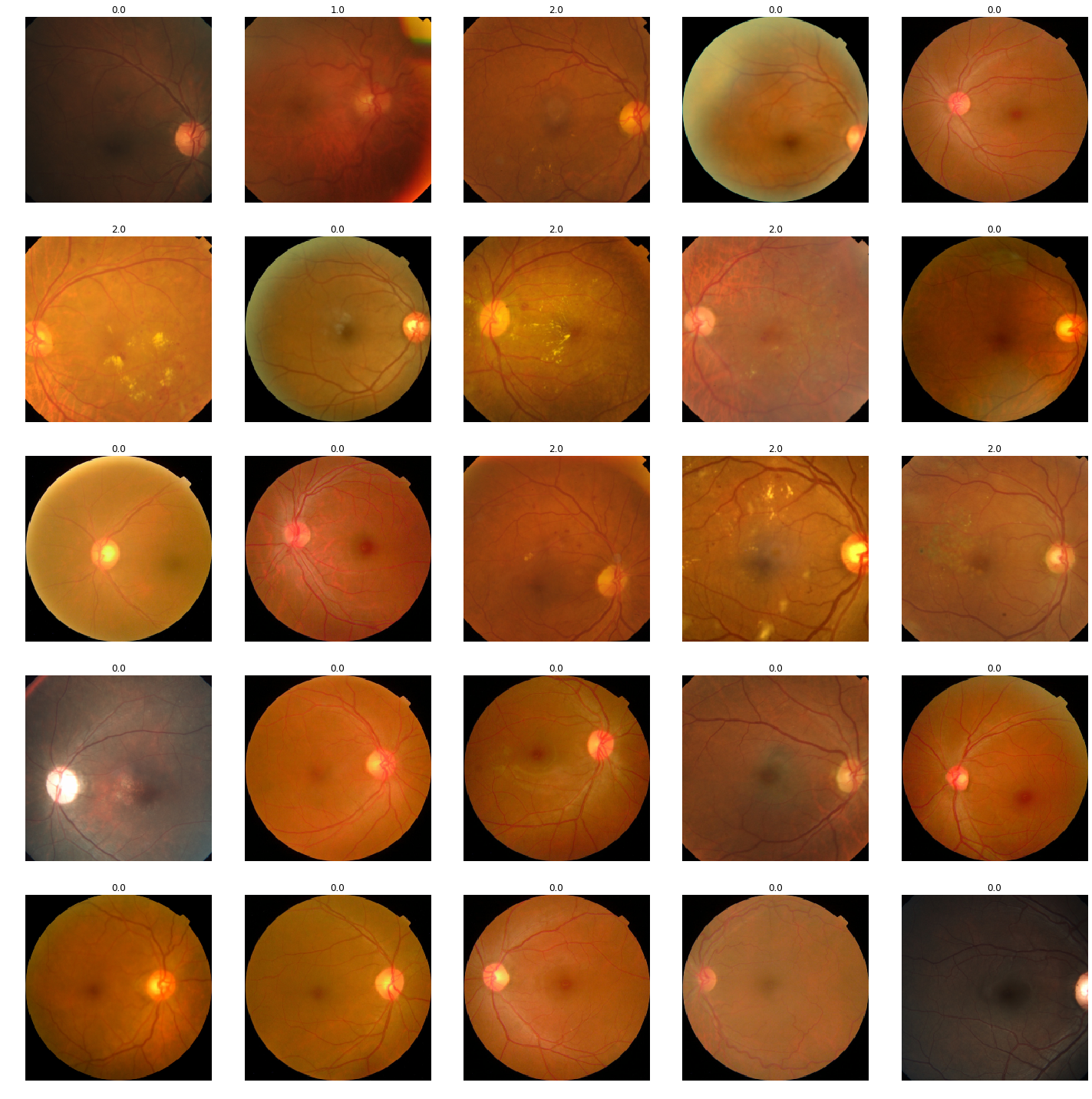
Before we start any training we try to get a good sense of the raw data, understand its distributions, and explore its features and idiosyncracies.
Getting to know our dataset is an important first step, and helps us tune our model towards more accurate predictions.
Loaded pretrained weights for efficientnet-b2
Using data in: /hdd/data/blindness-detection/2015_and_2019/train/
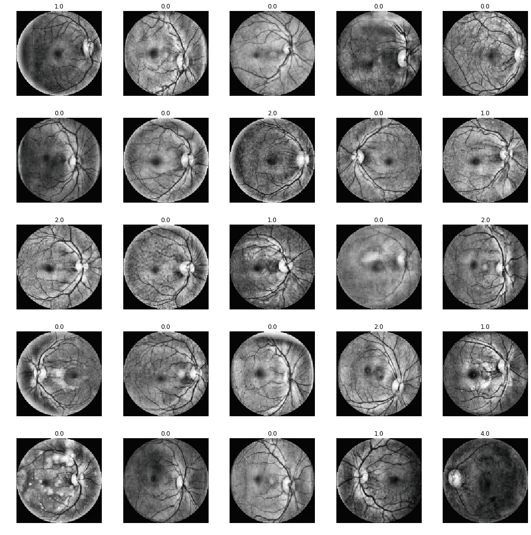
7.0.1 Inconsistent cropping and lighting
As we can see from the above images, the input images are inconsistently cropped, and is the product of coming from a variety of different sources, equipment quality, and time periods.
Another inconsistency is the lighting used in theses images.
We need to help improve the consistency of the images so that it helps the model work more effectvely. A start would be to get the cropping and lighting consistent across all of the images.
Let’s see what happens when we do some image processing:
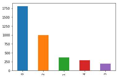
7.0.2 Data imbalance
We can see here that there is a definite data imbalance with the supplied data. A large percentage of the images coming through are actually normal, rather than containing any diabetic retinopathy.
We deal with this imbalance by oversampling the less dominant classes.
# checking for data imbalancesdata_in_use, base_dir, train_img_path, test_img_path, df_train = data_sourcecounts = df_train.diagnosis.value_counts() counts.plot(kind='bar')
8 Data Processing
To deal with the above problems, we tried to implement the following solutions to improve the input into the network.
8.1 Pre-resize
We first pre-resize our images into the sizes we want to give to our model. This gives us a signficant boost in trainign speed over resizing the images on the fly (say through a custom ItemList)
We create subfolders with resized versions of the images so we can retain the original images. When we resize the images, we also apply the various colour, cropping and image processing treatments so that we also do not have to perform them on the fly.
8.2 Image Preprocessing
Below I’ve explored various image processing strategies. The goal here was to normalise exposure, contrast and cropping as much as possile across the dataset to make it easier for our neural net to work on.
Filtering out the green channel was explored, along with various Gaussian filters and also various cropping tasks.
In the end we found that a simple colour and circle crop provided the best results.
The different processing methods that were explored can be seen below.
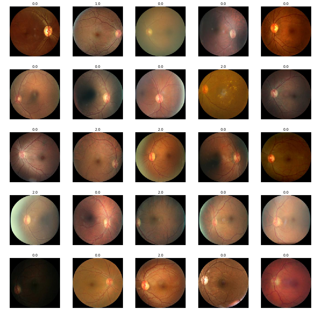
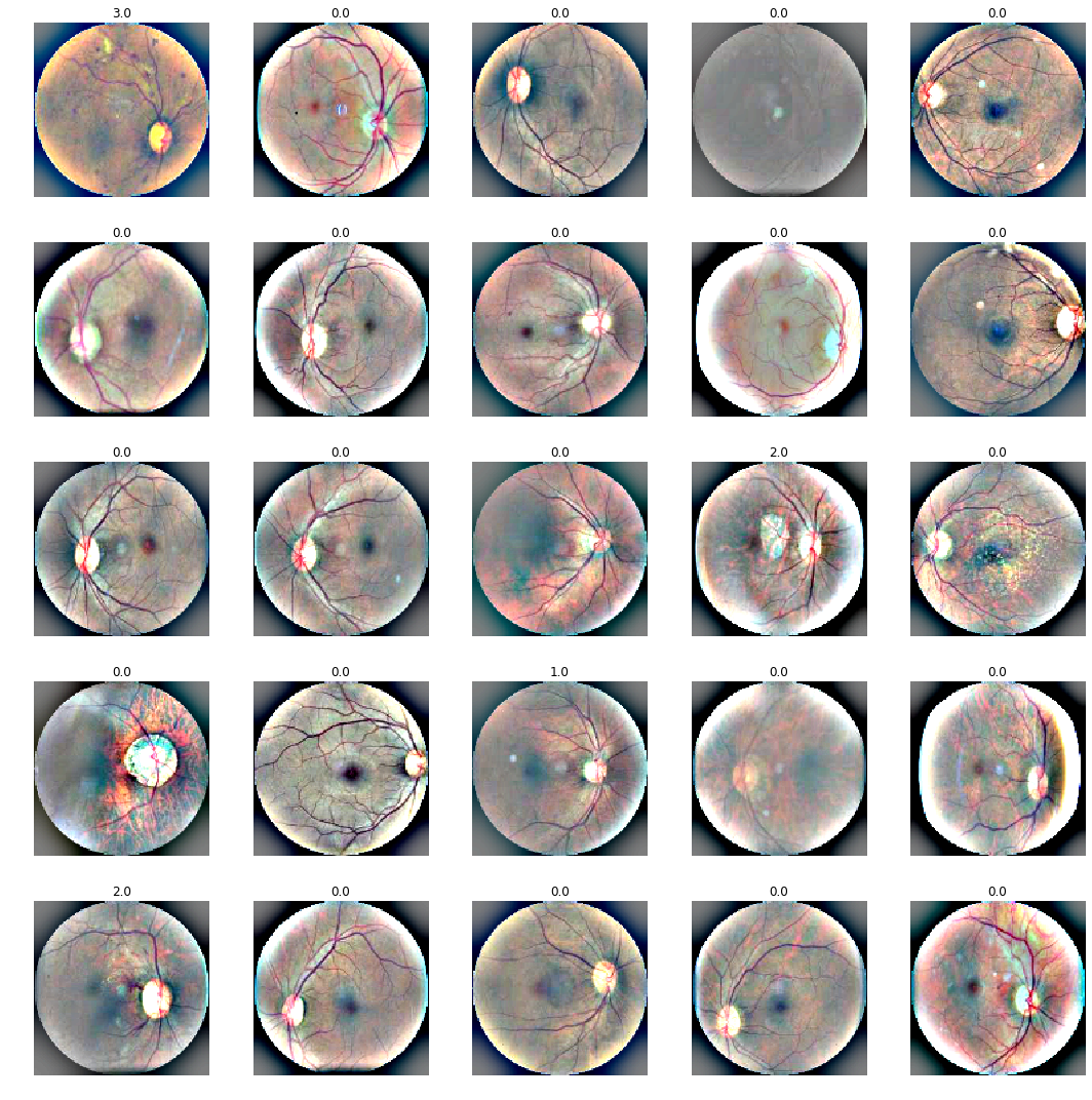
8.2.0.1 Circle crop and resize
The following image batch displays the image pre-processing that was eventually applied in our final training runs. These were a simple circle crop and resize, and standardising the black corners.
Using data in: /hdd/data/blindness-detection/2015_and_2019/train/224/
8.2.0.3 Green Channel Filter and Circle Crop
The paper here featured research around filtring out the green channel of the images to further highlight diabetic retinopathy indicators. http://biomedpharmajournal.org/vol10no2/diabetic-retinal-fundus-images-preprocessing-and-feature-extraction-for-early-detection-of-diabetic-retinopathy/
Although this provided good results, keeping the raw image colourisations seemed to work better in practice.
I also experimented with some cropping and gaussian colorisation filters that were outlined in the following kernel: https://www.kaggle.com/ratthachat/aptos-updatedv14-preprocessing-ben-s-cropping
Compared to using the raw colour vs green channel filter, vs Gaussian filter methods, we observed during training that that Gaussian filters actually resulted is visibly poorer results in training.
Using data in: /hdd/data/blindness-detection/2015_and_2019/train/224/
8.3 Oversample
Our dataset displays a class imbalance, a situation where there is a disproportionate amount of images classified to one particular class. In this case, there are a lot of images of healthy eyes in the dataset.
In order to give our model enough examples to learn to detect instances of diabetic retinpathy, we can try a technique called oversampling.
By oversampling we are in essence creating duplicates of our data. This creates a scenario where our network could start to overfit. We need to observe this and balance this out with some regularisation.
Even though the dataset was imbalanced, we found that oversampling introduced worse results.
9 TRAINING
Here we start looking at setting up our learners for training. As mentioned previously, training is performed offline, and the resulting models are then uploaded to Kaggle datasets and the kernel for inference on the public and private test set.
A summary of the key hyperparameters and setups that worked are listed below:
Fit one cycle policy for discriminitive learning rates.
Combine 2015 and 2019 datasets
Heavy data augmentations with cropping, lighting, and rotation.
Progressive resizing
Using EfficientNets: We explored a number of options for architectures. Including Resnets and Densenets. We found that EfficientNets provided the best results, so we use this with pretrained weights as our baseline architecture. https://arxiv.org/abs/1905.11946
Chose to approach this problem as a classifciation problem rather than a regression problem.
Adam optimiser.
Ensembling multiple models.
9.1 Classification or Regression
Try use CrossEntropyLoss and MSELoss (experiments not detailed below but I was able to determine previously that treating this as a regression problem gave best results).
9.2 More Data
Instead of training just on the 2019 dataset, we could use transfer learning and train on the 2015 dataset, and then use this as a pretrained network to train the 2019 dataset.
The other option was to combine both the 2015 and 2019 datasets into one large dataset.
This strategy provided the best results and generalised better on the private LB.
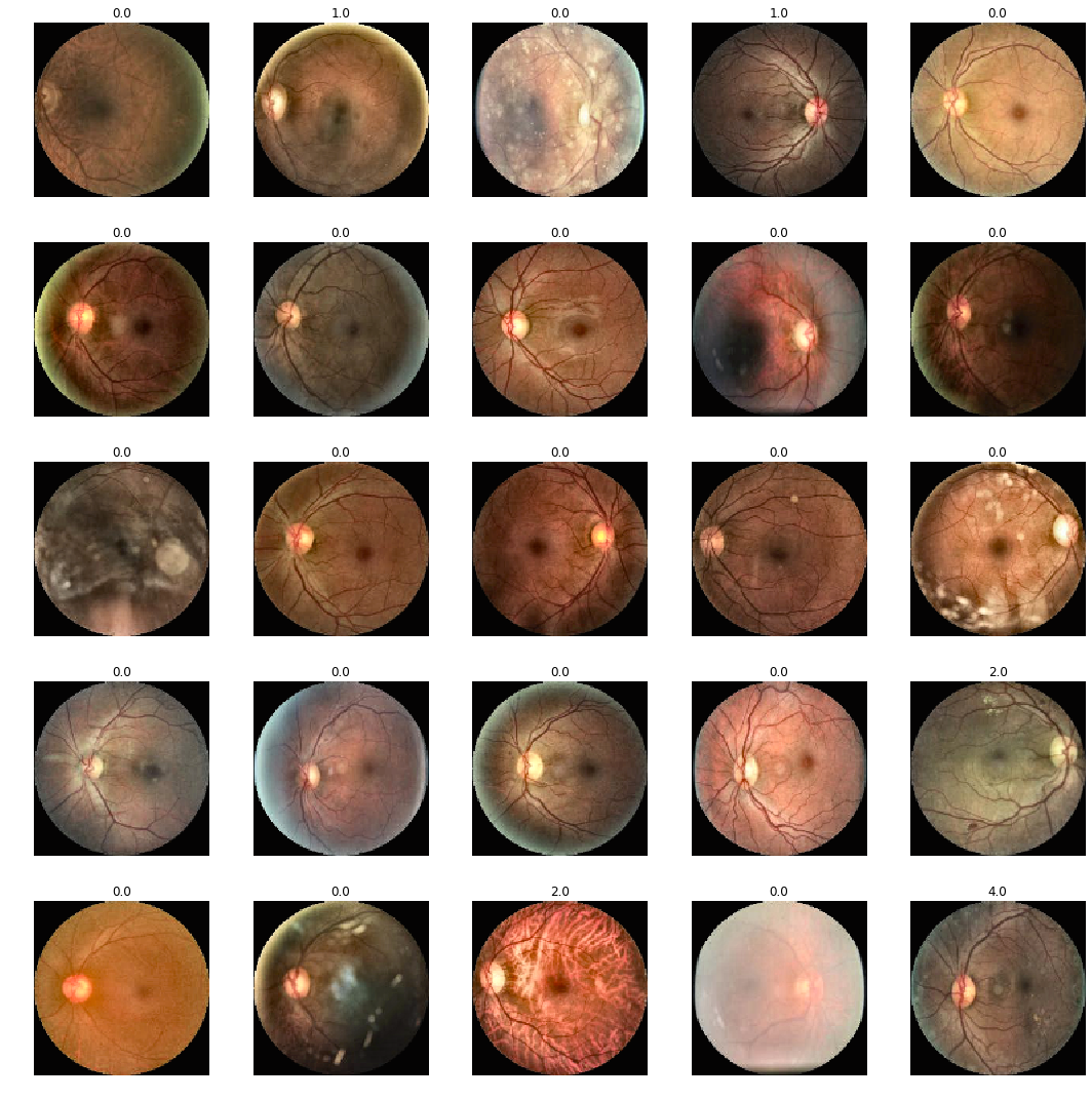
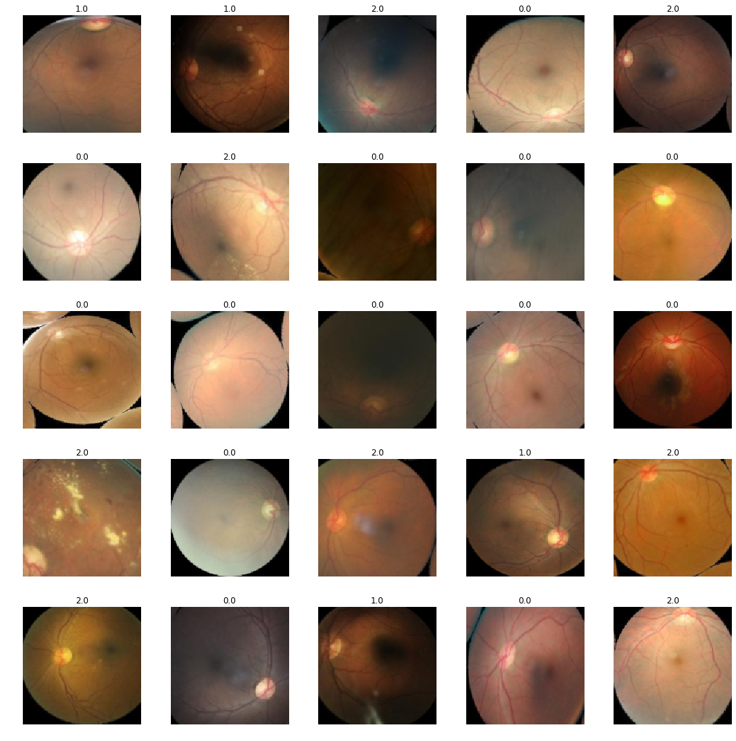
9.3 Data Augmentations
Data augmentations can be incredibly effective in improving machine learning models. Heavy augmentations seemed to help quite a lot in boosting accuracy in this competition.
In the original dataset we can see a lot of variability around lighting and cropping. We deal with this in one way through image pre-processing and standardising the original images. Another we deal with this is using data augmentation.
Along with serving as a means of regularisation and effectively increasing our dataset size, we also augment the data with a series of cropping, rotation, lighting, and zooming augmentations in an effort to smooth out the effect of the inconsistencies present in the photography of the original dataset.
The following displays the results of our augmentations.
Using data in: /hdd/data/blindness-detection/2015_and_2019/train/224/
9.4 Progressive Resizing
We get better results by starting with smaller images, and then gradually transfer learning to larger images. We start with a size of 224px for our training. Then feed the weights of these to the model trained against 352px images.
Loaded pretrained weights for efficientnet-b3
Using data in: /hdd/data/blindness-detection/2015_and_2019/train/224/
Using get_transforms
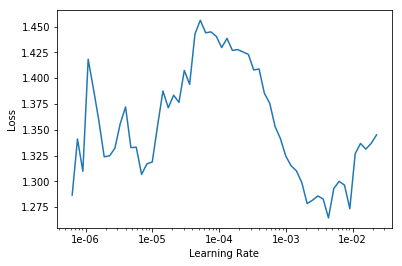
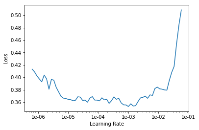
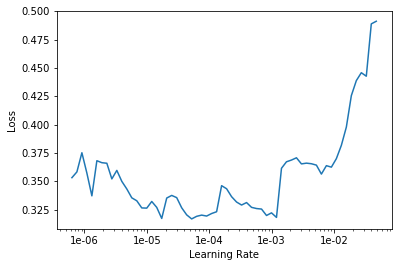
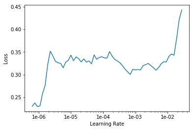
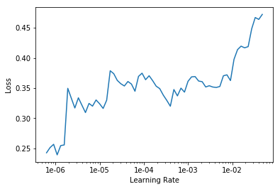
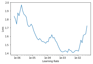
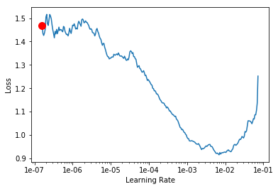
LR Finder is complete, type {learner_name}.recorder.plot() to see the graph.
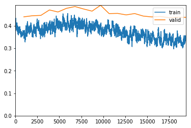
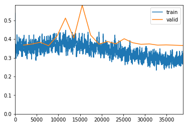
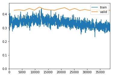
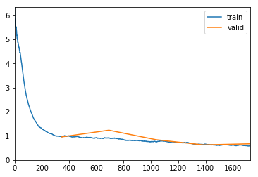
exp.fit_frozen(50, 2e-3)
epoch
train_loss
valid_loss
quadratic_kappa
time
0
0.685342
0.619710
0.545845
05:31
1
0.596974
0.571068
0.578879
05:38
2
0.618178
0.567687
0.588475
05:40
3
0.555176
0.585413
0.620093
05:39
4
0.593917
0.634622
0.600980
05:40
5
0.632227
0.587759
0.587736
05:41
6
0.644521
0.787938
0.440152
05:40
7
0.641000
0.667928
0.522046
05:43
8
0.622614
0.683303
0.533380
05:41
9
0.640435
0.953740
0.373591
05:40
10
0.638760
0.645746
0.534350
05:40
11
0.618202
0.751819
0.437967
05:41
12
0.590469
0.678545
0.539696
05:39
13
0.624134
0.625909
0.521491
05:41
14
0.601607
0.672399
0.473202
05:38
15
0.604112
0.596951
0.540873
05:40
16
0.571431
0.581151
0.573475
05:39
17
0.604839
0.605205
0.549892
05:38
18
0.578118
0.603482
0.576252
05:40
19
0.530020
0.685973
0.494106
05:43
20
0.583008
0.534397
0.620179
05:39
21
0.573428
0.613555
0.559092
05:43
22
0.532787
0.591532
0.560300
05:42
23
0.536919
0.641766
0.538613
05:39
24
0.492625
0.613391
0.585605
05:42
25
0.564835
0.556439
0.581119
05:42
26
0.517337
0.556271
0.604257
05:42
27
0.552688
0.534814
0.611220
05:40
28
0.518556
0.594337
0.591200
05:40
29
0.478324
0.550315
0.623366
05:40
30
0.465005
0.516290
0.633222
05:41
31
0.465429
0.575935
0.563715
05:41
32
0.459050
0.476072
0.659520
05:41
33
0.470096
0.478756
0.651597
05:43
34
0.466783
0.495208
0.640741
05:45
35
0.451121
0.475273
0.671176
05:44
36
0.424223
0.476628
0.665514
05:41
37
0.441065
0.500524
0.632676
05:42
38
0.437456
0.452326
0.681158
05:45
39
0.403897
0.494364
0.643641
05:43
40
0.367161
0.451442
0.673862
05:42
41
0.387677
0.449213
0.686294
05:45
42
0.421061
0.458739
0.668585
05:43
43
0.380013
0.435951
0.693150
05:44
44
0.389248
0.442668
0.686642
05:43
45
0.363035
0.443507
0.691067
05:43
46
0.388261
0.444286
0.688327
05:42
47
0.387743
0.442615
0.689882
05:44
48
0.372562
0.441129
0.692700
05:42
49
0.360547
0.440386
0.691759
05:43
Better model found at epoch 35 with valid_loss value: 0.4752731919288635.
Better model found at epoch 38 with valid_loss value: 0.4523259401321411.
Better model found at epoch 40 with valid_loss value: 0.4514419138431549.
Better model found at epoch 41 with valid_loss value: 0.44921305775642395.
Better model found at epoch 43 with valid_loss value: 0.4359509348869324.
exp.unfreeze()
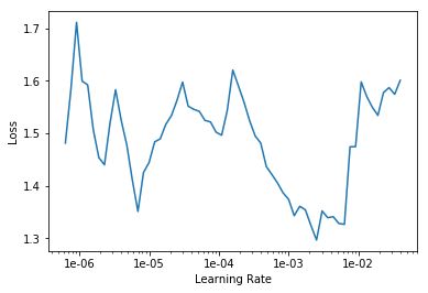
LR Finder is complete, type {learner_name}.recorder.plot() to see the graph.
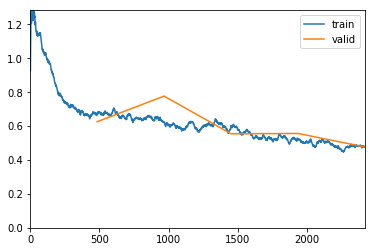
exp.fit_unfrozen(20, 2e-3/3)
epoch
train_loss
valid_loss
quadratic_kappa
time
0
0.355483
0.439657
0.688297
05:42
1
0.366197
0.444503
0.688321
05:45
2
0.375689
0.446104
0.685427
05:47
3
0.403844
0.470239
0.664926
05:42
4
0.408403
0.461219
0.676576
05:47
5
0.398039
0.477462
0.650838
05:45
6
0.418846
0.485373
0.637332
05:45
7
0.397980
0.474653
0.661722
05:46
8
0.418474
0.464985
0.679641
05:47
9
0.389099
0.491108
0.633804
05:46
10
0.380193
0.454011
0.674628
05:49
11
0.376623
0.454947
0.674366
05:47
12
0.377168
0.448288
0.673841
05:47
13
0.398294
0.454249
0.693535
05:45
14
0.373084
0.443102
0.688910
05:50
15
0.344921
0.439213
0.697587
05:47
16
0.321437
0.441183
0.688341
05:42
17
0.339580
0.436000
0.697186
05:45
18
0.363504
0.437782
0.694226
05:46
19
0.336848
0.437483
0.696593
05:44
Better model found at epoch 0 with valid_loss value: 0.43965739011764526.
Better model found at epoch 15 with valid_loss value: 0.4392130374908447.
Better model found at epoch 17 with valid_loss value: 0.43600040674209595.
Loaded pretrained weights for efficientnet-b3
Using data in: /hdd/data/blindness-detection/2015_and_2019/train/352/
Using get_transforms
Loading pretrained model: unf_exp_full_train_224_efficientnet-b3
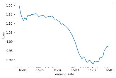
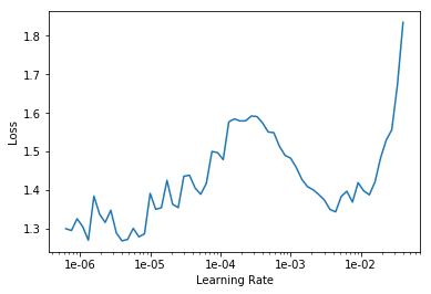
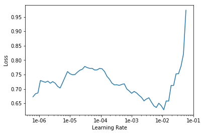
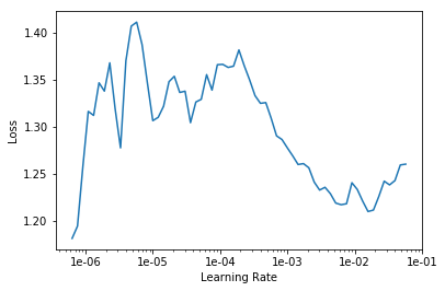
LR Finder is complete, type {learner_name}.recorder.plot() to see the graph.
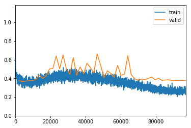
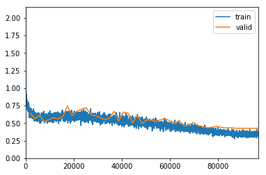
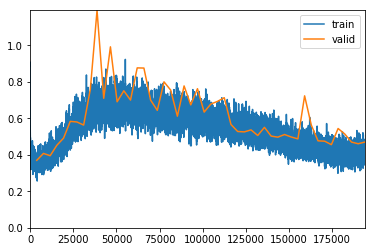
exp.fit_frozen(50, 1e-3)
epoch
train_loss
valid_loss
quadratic_kappa
time
0
0.378758
0.376949
nan
12:25
1
0.364224
0.365304
nan
12:36
2
0.382510
0.370127
0.713891
12:34
3
0.376226
0.373534
0.722537
12:35
4
0.371377
0.376860
nan
12:36
5
0.358835
0.385350
0.701696
12:37
6
0.401600
0.434859
nan
12:36
7
0.412164
0.399532
0.698118
12:37
8
0.390873
0.422254
0.666851
12:38
9
0.388066
0.500082
0.673931
12:41
10
0.437900
0.505949
nan
12:42
11
0.390991
0.640664
nan
12:36
12
0.455951
0.501692
nan
12:39
13
0.461126
0.650071
nan
12:38
14
0.400187
0.497508
0.618025
12:38
15
0.443355
0.445772
nan
12:31
16
0.434101
0.623643
0.568809
12:37
17
0.399546
0.431995
0.669738
12:35
18
0.451687
0.522574
nan
12:38
19
0.421694
0.447511
nan
12:39
20
0.423959
0.561190
nan
12:38
21
0.471017
0.517371
0.648686
12:40
22
0.422174
0.456127
0.691005
12:39
23
0.415511
0.661708
0.624388
12:42
24
0.413321
0.542787
nan
12:38
25
0.404340
0.407079
0.694435
12:40
26
0.395765
0.481117
0.629505
12:38
27
0.326620
0.453025
nan
12:40
28
0.408697
0.409218
nan
12:40
29
0.368440
0.537910
0.646179
12:39
30
0.329484
0.432478
nan
12:38
31
0.358978
0.444529
0.697926
12:33
32
0.363501
0.643090
0.707714
12:36
33
0.364408
0.438274
0.689685
12:40
34
0.346218
0.395282
0.716795
12:42
35
0.333619
0.381019
0.705948
12:35
36
0.282752
0.391902
0.722615
12:38
37
0.284697
0.385550
0.722432
12:40
38
0.295718
0.399403
0.722060
12:44
39
0.301479
0.414364
0.717080
12:38
40
0.275269
0.385260
0.716763
12:42
41
0.303773
0.399387
0.723052
12:37
42
0.251041
0.378457
0.728782
12:40
43
0.267637
0.382559
0.729941
12:42
44
0.270321
0.384342
0.725919
12:37
45
0.245405
0.376402
0.729031
12:42
46
0.261571
0.376969
0.733021
12:38
47
0.276336
0.375040
0.734086
12:41
48
0.246320
0.377162
0.736666
12:39
49
0.299888
0.374446
0.733259
12:39
/home/adeperio/anaconda3/lib/python3.7/site-packages/sklearn/metrics/classification.py:373: RuntimeWarning: invalid value encountered in true_divide
  k = np.sum(w_mat * confusion) / np.sum(w_mat * expected)
Better model found at epoch 0 with valid_loss value: 0.3769490420818329.
Better model found at epoch 1 with valid_loss value: 0.36530375480651855.
Loaded pretrained weights for efficientnet-b5
Using data in: /hdd/data/blindness-detection/2015_and_2019/train/224/
Using get_transforms
LR Finder is complete, type {learner_name}.recorder.plot() to see the graph.
exp.fit_frozen(50, 1e-3)
epoch
train_loss
valid_loss
quadratic_kappa
time
0
0.595345
0.646250
0.475005
13:00
1
0.592122
0.560756
0.556119
13:03
2
0.543716
0.610841
0.501747
13:00
3
0.605076
0.524397
0.585637
13:01
4
0.583582
0.547083
0.590754
13:00
5
0.609600
0.578056
0.533149
13:01
6
0.577295
0.559897
0.597622
13:06
7
0.597799
0.591496
0.509156
13:06
8
0.616400
0.743248
nan
13:02
9
0.626760
0.606392
0.547063
13:03
10
0.602613
0.668969
nan
13:02
11
0.645009
0.696823
0.424927
13:02
12
0.610261
0.720009
0.513902
13:07
13
0.579437
0.622490
nan
13:04
14
0.577785
0.604873
0.503102
13:03
15
0.538940
0.578461
0.539171
13:06
16
0.544767
0.546279
0.578014
13:08
17
0.537881
0.570902
0.597600
13:10
18
0.511949
0.670403
nan
13:07
19
0.522222
0.529480
0.597809
13:08
20
0.528282
0.657377
0.602783
13:10
21
0.508090
0.639336
nan
13:09
22
0.538038
0.504943
0.623391
13:13
23
0.587688
0.612449
0.541492
13:11
24
0.500340
0.493437
0.623449
13:14
25
0.515066
0.544601
0.618239
13:10
26
0.488631
0.543157
0.567873
13:08
27
0.523809
0.523644
nan
13:15
28
0.453457
0.548754
nan
13:13
29
0.456395
0.566812
0.642520
13:09
30
0.412951
0.528970
nan
13:08
31
0.537828
0.498892
nan
13:07
32
0.423157
0.536432
nan
13:07
33
0.386358
0.458569
0.629433
13:06
34
0.461502
0.469598
0.644802
13:06
35
0.388960
0.509905
0.612689
13:08
36
0.417862
0.464479
nan
13:08
37
0.418502
0.453347
0.647451
13:09
38
0.406408
0.434712
0.666715
13:07
39
0.381572
0.440594
0.644749
13:07
40
0.382604
0.452715
nan
13:08
41
0.370123
0.441038
0.665932
13:07
42
0.376259
0.431814
0.654034
13:10
43
0.329282
0.434962
0.658811
13:07
44
0.359504
0.426874
0.668100
13:08
45
0.357846
0.426276
0.668389
13:09
46
0.359646
0.426947
0.671260
13:09
47
0.359240
0.426201
0.665448
13:10
48
0.326063
0.426390
0.665145
13:09
49
0.371072
0.427722
0.663822
13:08
Better model found at epoch 0 with valid_loss value: 0.6462504267692566.
Better model found at epoch 1 with valid_loss value: 0.560756266117096.
Better model found at epoch 3 with valid_loss value: 0.524396538734436.
/home/adeperio/anaconda3/lib/python3.7/site-packages/sklearn/metrics/classification.py:373: RuntimeWarning: invalid value encountered in true_divide
  k = np.sum(w_mat * confusion) / np.sum(w_mat * expected)
Better model found at epoch 33 with valid_loss value: 0.4585687518119812.
Better model found at epoch 37 with valid_loss value: 0.45334669947624207.
Better model found at epoch 38 with valid_loss value: 0.4347122013568878.
Better model found at epoch 42 with valid_loss value: 0.4318144917488098.
Better model found at epoch 44 with valid_loss value: 0.4268737733364105.
Better model found at epoch 45 with valid_loss value: 0.42627590894699097.
Better model found at epoch 47 with valid_loss value: 0.4262005686759949.
Loaded pretrained weights for efficientnet-b5
Using data in: /hdd/data/blindness-detection/2015_and_2019/train/352/
Using get_transforms
Loading pretrained model: unf_exp_full_train_224_efficientnet-b5
LR Finder is complete, type {learner_name}.recorder.plot() to see the graph.
9.10.1 (B5) Frozen 352 Training
exp.fit_frozen(50, 3e-3)
epoch
train_loss
valid_loss
quadratic_kappa
time
0
0.296111
0.370104
nan
27:12
1
0.313915
0.407937
nan
27:16
2
0.329492
0.395435
nan
27:21
3
0.515533
0.452583
nan
27:18
4
0.486743
0.491821
nan
27:21
5
0.448745
0.583675
nan
27:14
6
0.632567
0.580358
nan
27:17
7
0.568568
0.563487
nan
27:19
8
0.652277
0.760102
nan
27:12
9
0.640356
1.192581
0.238264
27:16
10
0.809779
0.710387
nan
27:15
11
0.669706
0.992560
nan
27:12
12
0.735946
0.691278
nan
27:12
13
0.740307
0.751535
nan
27:19
14
0.665691
0.700673
0.276416
27:22
15
0.706394
0.877093
0.368763
27:22
16
0.657666
0.876099
nan
27:29
17
0.684086
0.700442
0.263370
27:33
18
0.582564
0.644197
nan
27:26
19
0.583665
0.800478
nan
27:26
20
0.638894
0.755252
nan
27:30
21
0.578587
0.612095
nan
27:42
22
0.631876
0.778131
nan
27:45
23
0.539442
0.674228
nan
27:41
24
0.537807
0.762890
0.273097
27:40
25
0.574273
0.634675
nan
27:49
26
0.598411
0.679090
0.302701
28:01
27
0.657017
0.693446
nan
27:50
28
0.594459
0.713499
0.414432
27:46
29
0.459683
0.566890
nan
27:48
30
0.521934
0.528279
nan
27:55
31
0.560276
0.526069
nan
27:58
32
0.505221
0.537023
nan
27:49
33
0.524495
0.506361
nan
28:01
34
0.503538
0.550988
nan
28:00
35
0.522662
0.503027
nan
28:01
36
0.432941
0.497164
nan
28:02
37
0.454244
0.511560
nan
28:08
38
0.500142
0.498066
nan
28:08
39
0.450399
0.487739
nan
28:06
40
0.522259
0.723720
0.454567
28:06
41
0.392952
0.563218
nan
28:07
42
0.441279
0.477039
nan
28:05
43
0.405745
0.475012
nan
28:12
44
0.427733
0.455954
nan
28:15
45
0.384656
0.544580
nan
28:16
46
0.458088
0.514241
nan
28:16
47
0.415536
0.470183
nan
28:20
48
0.373178
0.461036
nan
28:21
49
0.391088
0.470336
nan
28:18
/home/adeperio/anaconda3/lib/python3.7/site-packages/sklearn/metrics/classification.py:373: RuntimeWarning: invalid value encountered in true_divide
k = np.sum(w_mat * confusion) / np.sum(w_mat * expected)
Better model found at epoch 0 with valid_loss value: 0.37010443210601807.
Inference is performed directly in a Kaggle kernel after uploading the trained models to a Kaggle private dataset.
Before we perform inference, the test set has not been pre-processed like the images in our training set.
So here we use a custom Fastai ItemList (CleanedImageList) and apply the same image pre-processing the images in our test set (circle crop, resize). If we don’t do this our predictions will be significantly off.
A number of experiments were performed to determine the best hyper paramters for the network. Below are some of the key experiments that were performed, detailed to highlight experimental process and work flow.
First we encapsulated experiment hyper paramaters in an “Experiment” class.
Then for each experiment, we create a “baseline” function that intialises a set of hyper parameters that we want to remain constant, but takes as function paramaters then hyper parameters we are trying to test.
Then we run over a small number of epochs to get a rough indiciation of what best works.
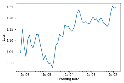
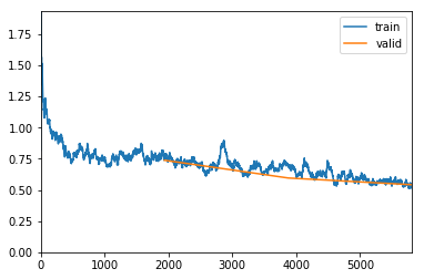
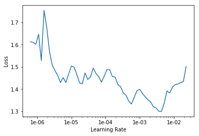
14.1 (Exp-1) Batch Size vs Model Complexity
14.1.0.1 Summary
The following experiment tries to observe the performance of changing batch size vs model complexity.
Comparing for batch size - efficientnet-b2 and bs=64 - efficientnet-b2 and bs=16
We can see that higher batch sizes have better accuracy
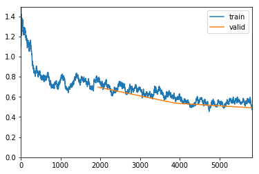
Comparing for model complexity - efficientnet-b2 and bs=16 - efficientnet-b5 and bs=16
We can see that the more complex b5 also gets better accuracy, and even better than the b2 with bs=16.
So we use b5 as one of our ensemble models to train from.
But increasing model complexity also brings up the accuracy even with lower batch sizes.
Loaded pretrained weights for efficientnet-b2
Using data in: /hdd/data/blindness-detection/2015_and_2019/train/224/
Using get_transforms
LR Finder is complete, type {learner_name}.recorder.plot() to see the graph.
exp.fit_frozen(3, 1e-4)
epoch
train_loss
valid_loss
quadratic_kappa
time
0
0.677559
0.702017
0.564117
03:24
1
0.587030
0.569272
0.654701
03:35
2
0.524190
0.500103
0.648396
03:36
Better model found at epoch 0 with valid_loss value: 0.7020165920257568.
Better model found at epoch 1 with valid_loss value: 0.5692717432975769.
Better model found at epoch 2 with valid_loss value: 0.500103235244751.
Loaded pretrained weights for efficientnet-b2
Using data in: /hdd/data/blindness-detection/2015_and_2019/train/224/
Using get_transforms
LR Finder is complete, type {learner_name}.recorder.plot() to see the graph.
exp.fit_frozen(3, 1e-3)
epoch
train_loss
valid_loss
quadratic_kappa
time
0
0.752668
0.737975
nan
09:15
1
0.692548
0.595446
0.515833
09:23
2
0.514083
0.541481
0.563979
09:22
/home/adeperio/anaconda3/lib/python3.7/site-packages/sklearn/metrics/classification.py:373: RuntimeWarning: invalid value encountered in true_divide
k = np.sum(w_mat * confusion) / np.sum(w_mat * expected)
Better model found at epoch 0 with valid_loss value: 0.7379746437072754.
Better model found at epoch 1 with valid_loss value: 0.5954458117485046.
Better model found at epoch 2 with valid_loss value: 0.541480541229248.
Loaded pretrained weights for efficientnet-b5
Using data in: /hdd/data/blindness-detection/2015_and_2019/train/224/
Using get_transforms
LR Finder is complete, type {learner_name}.recorder.plot() to see the graph.
exp.fit_frozen(3, 5e-4)
epoch
train_loss
valid_loss
quadratic_kappa
time
0
0.750439
0.696666
0.508375
12:51
1
0.582432
0.537899
0.561278
13:00
2
0.475572
0.491343
0.604045
13:01
Better model found at epoch 0 with valid_loss value: 0.69666588306427.
Better model found at epoch 1 with valid_loss value: 0.5378988981246948.
Better model found at epoch 2 with valid_loss value: 0.49134281277656555.
14.2 (Exp-2) Progressive Resize
14.2.0.1 Summary
We pretrained 224px on 2015 and 2019 data.
Then we used this to progressize resize to 352, and only on the 2019 data.
This resulted in a significant boost to our CV score.
Loaded pretrained weights for efficientnet-b5
Using data in: /hdd/data/blindness-detection/2015_and_2019/train/352/
Using get_transforms
Loading pretrained model: exp2_bs16_224_efficientnet-b5
LR Finder is complete, type {learner_name}.recorder.plot() to see the graph.
exp.fit_frozen(3, 5e-4)
epoch
train_loss
valid_loss
quadratic_kappa
time
0
0.717716
1.350634
0.578072
02:31
1
0.489375
0.328841
0.840936
02:32
2
0.369162
0.304662
0.857985
02:32
Better model found at epoch 0 with valid_loss value: 1.3506337404251099.
Better model found at epoch 1 with valid_loss value: 0.32884085178375244.
Better model found at epoch 2 with valid_loss value: 0.3046622574329376.
14.3 (Exp-3) Oversample vs Non-Oversample
14.3.0.1 Summary
As we can clearly see, although there was an imbalance with the dataset, oversampling gave significantly poorer results.
We turn Oversampling off on our main training run.
Loaded pretrained weights for efficientnet-b2
Using data in: /hdd/data/blindness-detection/2015_and_2019/train/224/
Using get_transforms
is oversampling
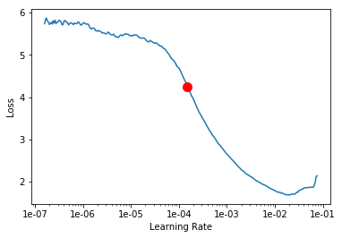
LR Finder is complete, type {learner_name}.recorder.plot() to see the graph.
Min numerical gradient: 1.51E-04
Min loss divided by 10: 2.00E-03
exp.fit_frozen(5, 1e-3)
epoch
train_loss
valid_loss
quadratic_kappa
time
0
0.969762
0.956943
0.442457
02:33
1
0.919834
1.236394
0.525234
02:37
2
0.762089
0.841168
0.463579
02:39
3
0.643005
0.626805
0.585560
02:37
4
0.575614
0.672715
0.555053
02:38
Better model found at epoch 0 with valid_loss value: 0.9569430351257324.
Better model found at epoch 2 with valid_loss value: 0.8411678671836853.
Better model found at epoch 3 with valid_loss value: 0.6268053650856018.
Loaded pretrained weights for efficientnet-b2
Using data in: /hdd/data/blindness-detection/2015_and_2019/train/224/
Using get_transforms
LR Finder is complete, type {learner_name}.recorder.plot() to see the graph.
Min numerical gradient: 1.58E-07
Min loss divided by 10: 6.92E-04
exp.fit_frozen(5, 1e-3)
epoch
train_loss
valid_loss
quadratic_kappa
time
0
0.672804
0.625812
0.549030
03:35
1
0.623003
0.776893
0.600862
03:35
2
0.596965
0.554515
0.580464
03:36
3
0.523275
0.556523
0.601181
03:35
4
0.477067
0.476698
0.667192
03:35
Better model found at epoch 0 with valid_loss value: 0.6258118152618408.
Better model found at epoch 2 with valid_loss value: 0.5545154213905334.
Better model found at epoch 4 with valid_loss value: 0.47669753432273865.
Google work on diabetic retiopathy: - https://ai.googleblog.com/2018/12/improving-effectiveness-of-diabetic.html - https://ai.googleblog.com/2016/11/deep-learning-for-detection-of-diabetic.html
Image processing: - bens original - https://www.kaggle.com/ratthachat/aptos-updatedv14-preprocessing-ben-s-cropping - circle cropping https://www.kaggle.com/taindow/pre-processing-train-and-test-images - Paper on focusing on green channel for most information http://biomedpharmajournal.org/vol10no2/diabetic-retinal-fundus-images-preprocessing-and-feature-extraction-for-early-detection-of-diabetic-retinopathy/ - Green channel post on discussion board - https://www.kaggle.com/c/aptos2019-blindness-detection/discussion/102613#latest-598093